The Visualization Process – It Starts with the Data

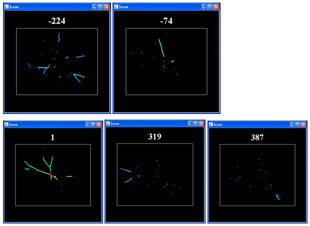
Figure 1 – Neuron image cross sections, the real raw data

How the Data was Gathered:

Knowing how the data was gathered can give insight to its nature and provide details. The data gathering process, for this data set, was explained to us as follows: “The motor neurons were filled with a dye and then the spinal cord was cut into cross sections, each with a thickness of 50 microns. Since the dendrites extend for almost 2000 microns away from the cell body, about 80 cross sections were needed to reconstruct one motor neuron. A computer-microscope system was then used to map the x and y coordinates of the dendritic tree in each section, and it also provided the z coordinate. The diameter of the dendritic tree at each coordinate was measured using a magnification of 1,000 times.”

Putting the Slices Together:

The position and diameter data for the dendrites were manually measured from the images using a microscope. This resulted in a set of coordinates (x, y, z) for each end of a segment of the dendrite, along with a diameter for that segment of the dendrite.

To construct a visual representation we can just connect the (x, y, z) coordinate dots together. When we colour the dendrite sections by the diameter, we get the image of Fig. 2:

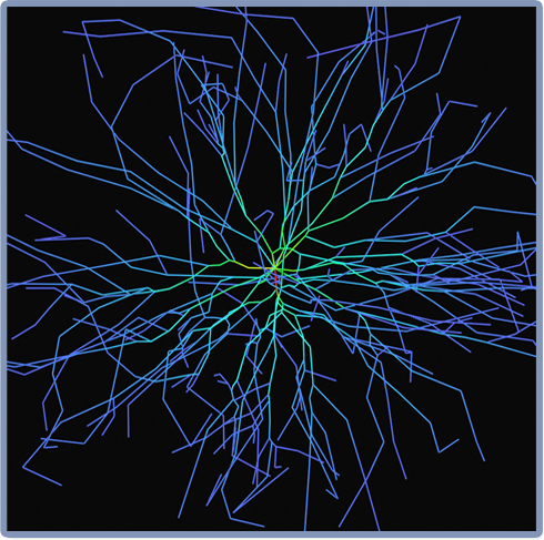
Figure 2 – Neuron data connected by line segments. (The color indicates the diameter of the dendrites.)

Smoothing the Data:

Point-to-point connection of the measured dendrite segments created an artificial crinkled structure resulting from the limited number of measurements made and the thickness of the sections. However, the dendrite geometry seen in a microscope has a smoothly curving trajectory.

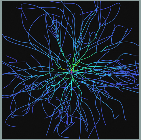
Figure 3 – Neuron data connected with splines

A numerical smoothing algorithm was used to approximate the realistic shape between the measured points. Specifically, cubic splines were used to remove the “kinks” in the data and create a smooth geometry more like the original nerve cells.

Adding a Reference Structure

Next a sphere and line has been added to represent structures in the centre of the neuron that were not included in the original data. The sphere has the same surface area as the irregular cell body measured with a microscope. The line represents the initial segment of the axon that will exit the spinal cord and connect the motor neuron to a muscle.

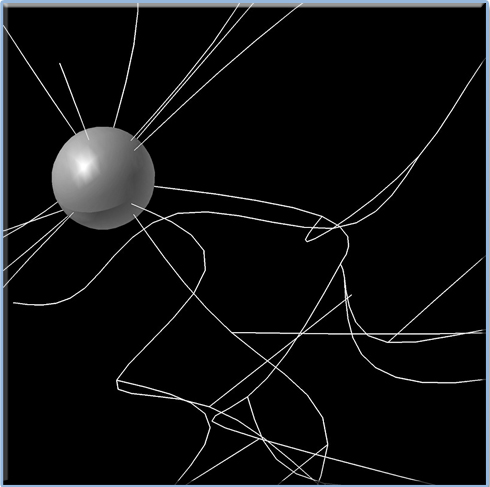
Figure 4 – Neuron with cell body.

A Geometric Model:

Real dendrites are not just thin lines with a uniform thickness, the thickness varies from the cell body to the tip. Fortunately the data included measurements of the diameter of each dendrite at various points along its length. This allows the colour used in Fig. 2 to be replaced by a three dimensional surface.

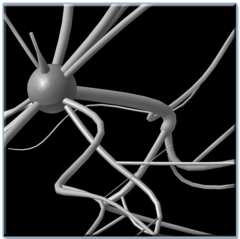
Figure 5 – Dendrites with varying thickness.

The resulting geometry was used as a basis for a three dimensional model to visualize the results of numerical simulations of the electrical behaviour of these cells.

Visuals for the Web:

Although the primary goal of the project was to create the geometry for use in numerical simulations, a benefit of having the geometry allows for the output to be presented in a number of forms. Here we are featuring a WebGL version of the data (for details on using WebGL see “Interacting with WebGL On This Site”):

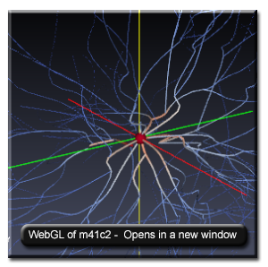
Figure 6 – Motor Neuron M41C2

(Project initiated at the University of Alberta and continued with Videre Analytics, 2014. The original programming for this project was done by Maryia Kazakevitch, then at the University of Alberta. The information here was adapted from: Scientific Visualization and Rendering of Motor Neurons, Principle Investigator: Dr. Kelvin Jones, Faculty of Physical Education and Recreation, University of Alberta.)