
Visualization of Quantum States
[layerslider id=”1″]
The purpose of this article is not to explain quantum mechanics in detail, but rather to demonstrate that 3D visualization can assist with understanding complex topics. The mathematics of quantum mechanics is interesting in its own right, but with the aid of suitable visualizations, the content can be understood by the viewer, and that understanding shared with others.
The hydrogen atom is composed of two particles, the electron, a negatively charged particle, and the proton, a positively charged particle, bound together into a stable system. The proton is relatively heavy compared to the electron so a simple picture of the system is natural: the proton is in the centre of the electron-proton system and the electron moves around the proton in almost circular orbits. This solar-system-like picture of atoms is helpful in explaining the qualitative structure, but it doesn’t work when we want to actually calculate properties of atoms. For that we need a more detailed picture provided by the mathematics of quantum mechanics.
In quantum mechanics, an object is described by a “wave function” which describes everything about the object. The wave function of an object is related to the probability that the object is going to be found in a region of space. If we are describing the object without taking the effects of relativity into account, the wave function is the solution of the time independent Schrödinger equation
$$ H \Psi = E \Psi$$
The \(H\) is a differential operator that varies with the system under consideration, and can be quite complicated, and E is the energy of the wave function (or state) that solves the equation. In this discussion we are only interested in states that don’t change with time.
The solutions of the Schrödinger Equation for the electron-proton system are in two pieces multiplied together: the first depends on the distance the electron is away from the origin, and the second piece depends on the angular position of the electron in the coordinate system. The solution can be written as
$$\Psi_{nlm} = R_{nl}(r) Y_{lm}(\theta, \phi)$$
The quantum nature of quantum mechanics enters with the realization that there are solutions to this problem only when \(n\), \(l\) and \(m\) are integers. There are some other conditions on these “quantum numbers”, but for our purposes, all we will care about are some of the sets of quantum numbers. The position of the electron around the proton isn’t described by a circular orbit at all, as you might have pictured when we mentioned the planetary model earlier. In fact there is some probability that the electron can be anywhere in space. The regions where the electron spends most of its time varies as the quantum numbers change, and we would like to understand this a bit.
As the values of the quantum numbers increase, the electron spends more time further away from the proton. The WebGL view in Figure 1 demonstrates this by showing three states together: (1,0,0) – green, (2,1,1) – red and (3,2,1) – blue. The surfaces for each enclose the space where the electron spends half of its time while in that particular state. As you can see, the electron is spending its time in quite different regions of space as the quantum number increase. These higher levels are “excited states” in which the electron has absorbed a specific amount of energy and angular momentum to make the transition to that state. The rules governing quantum numbers and transitions can be found in texts on quantum mechanics – the point here is that we understand the relationships much more easily when we can see them. The visual processing part of our brain is large compared to anything else the brain does, and harnessing that is very helpful in understanding data.
Figure 1 – Three states of the hydrogen atom: (n,l,m) = (1,0,0), (2,1,1) and (3,2,1). This is WebGL so you can grab it with the left mouse button to rotate it.
We have created 3D WebGL views of some hydrogen states. These currently work best in the Google Chrome browser – see the page “Interacting with WebGL On This Site”.
For the specific states, i.e. a single set of quantum numbers \(n, l, m\), the innermost surface, shown in red, encloses the region of space where the electron spends 10% of its time. The outermost surface, shown in blue, encloses the region of space where the electron spends 90% of its time. There are surfaces with levels in between, where the electron spends 30%, 50% and 70% of its time. These intermediate surfaces have different colors because their position on the color scale will vary, but the surfaces contain the volumes with the indicated probability. We only show half of the objects, a vertical slice has been taken so we can see into the objects.
Clicking on the images of hydrogen states below will open a new browser tab containing the WebGL object to interact with.
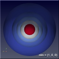
Figure 2(a) – Hydrogen ground state: (1, 0, 0). Download size – 600 KB.
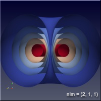
Figure 2(b) – Hydrogen state: (2, 1, 1). Download size – 5.4 MB.
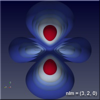
Figure 2(c) – Hydrogen state: (3, 2, 0). Download size – 11.8 MB.
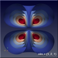
Figure 2(d) – Hydrogen state: (3, 2, 1). Download size – 12.3 MB.
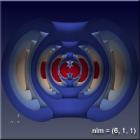
Figure 2(e) – Hydrogen state: (6, 1, 1). Download size – 13.1 MB.
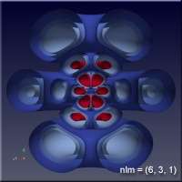
Figure 2(f) – Hydrogen state: (6, 3, 1). Download size – 7.5 MB.
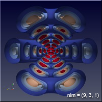
Figure 2(g) – Hydrogen state: (9, 3, 1). Download size – 71 MB (so be patient).
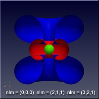
Figure 2(h) – Three hydrogen states: (0,0,0), (2,1,1) and (3, 2, 1). Download size – 3.3 MB.
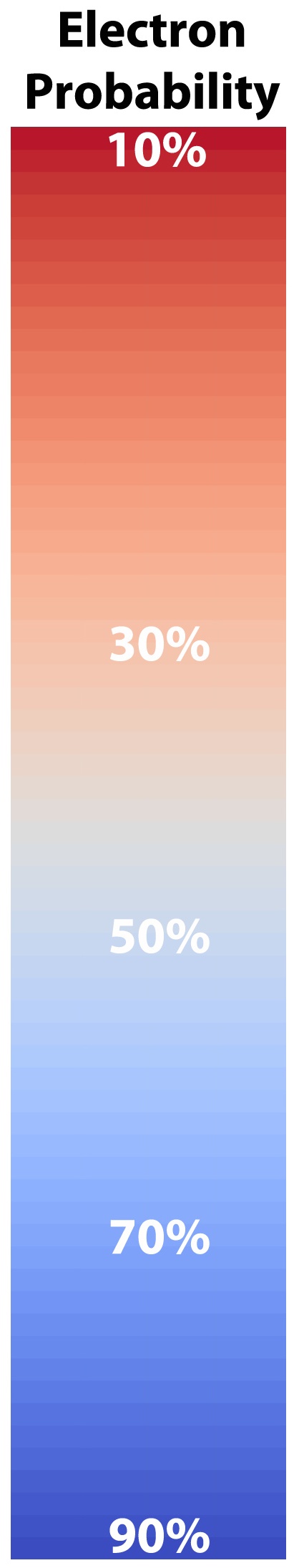
Figure 3 – Probability of finding the electron in a region of space in the hydrogen atom.